Viper: A High-Performance I/O Framework for Transparently Updating, Storing, and Transferring Deep Neural Network Models

@inproceedings{ye2024viper,
  title={Viper: A High-Performance I/O Framework for Transparently Updating, Storing, and Transferring Deep Neural Network Models},
  author={Ye, Jie and Cernuda, Jaime and Rajesh, Neeraj and Bateman, Keith and Yildiz, Orcun and Peterka, Tom and Nigmetov, Arnur and Morozov, Dmitriy and Sun, Xian-He and Kougkas, Anthony},
  booktitle={Proceedings of the 53rd International Conference on Parallel Processing},
  pages={812--821},
  year={2024}
}

Viper: A High-Performance I/O Framework for Transparently Updating, Storing, and Transferring Deep Neural Network Models

CCS CONCEPTS

• Computer systems organization → Neural networks; • Software and its engineering → Publish-subscribe / event-based architectures.

KEYWORDS

AI Workflows, Coupled Training and Inferences, Adaptive AI Model Checkpointing, Inferences During Partial Training

This work is licensed under a Creative Commons Attribution International 4.0 License.

ICPP '24, August 12-15, 2024, Gotland, Sweden

©2024 Copyright held by the owner/author(s).

ACM ISBN 979-8-4007-1793-2/24/08 https://doi.org/10.1145/3673038.3673070

ACM Reference Format:

Jie Ye, Jaime Cernuda, Neeraj Rajesh, Keith Bateman, Orcun Yildiz, Tom Peterka, Arnur Nigmetov, Dmitriy Morozov, Xian-He Sun, Anthony Kougkas, and Bogdan Nicolae. 2024. Viper: A High-Performance I/O Framework for Transparently Updating, Storing, and Transferring Deep Neural Network Models. In The 53rd International Conference on Parallel Processing (ICPP '24), August 12-15, 2024, Gotland, Sweden. ACM, New York, NY, USA, 10 pages. https://doi.org/10.1145/3673038.3673070

1 INTRODUCTION

Motivation: Deep Learning (DL) has attracted significant attention due to its robust and powerful capacity to extract insights from available data. Integrating Deep Learning (DL) with traditional High Performance Computing (HPC) simulations has shown significant promise in accelerating scientific discoveries [2]. Many scientific workflows employ DL at least partially: climate modeling [22], particle physical simulations [3], computational fluid dynamics [27], and virtual drug response prediction [29].

Traditionally, DL is employed in offline fashion, i.e., the learning model is pre-trained, and then used for inferences in the application workflow. However, offline DL is often insufficient, especially when the learning patterns are specific to individual workflow runs or when they fluctuate during the workflow execution [6], prompting the need to train and/or refine learning models on-the-fly. In this case, a naive solution that pauses the workflow during the training/fine-tuning leads to unacceptable runtime overhead and/or missed opportunities due to real-time constraints.

For example, consider the case of Ptychographic image reconstruction [1], which studies an unknown object by subjecting it to a high-intensity photon beam. As the beam passes through the object, it creates diffraction patterns that are captured by a sensor (at the edge) and analyzed further (on a remote HPC machine) to obtain the equivalent of an X-ray image at a small scale (e.g., molecular level). To reduce the transfer overhead between the edge and the HPC machine, generative learning models (e.g., PtychoNN [1]) are used to pre-process the diffraction patterns. However, each object is unique and the beam cannot be stopped. Therefore, we cannot use pre-trained model or pause the workflow until we trained one. Instead, we need to apply an online solution consisting of the following steps: (1) training warm-up: transfer the full diffraction patterns to the HPC machine, use a classic (but expensive) algorithm to reconstruct the images, while at the same time training a learning model using these images as ground truth; (2) switch to inferences: as soon as the learning model is accurate enough, transfer it to the edge and use it to pre-process the diffraction patterns; (3) fine-tuning: continue receiving a subset of the full diffraction patterns, refine the learning model (continue the training), and periodically send a checkpoint of the model to the edge to improve the quality of the inferences.

Implementing such a dynamic learning solution in HPC workflows is subject to two important questions: (1) how often to checkpoint a model during the fine-tuning step to improve the quality of the inferences; (2) how to design efficient techniques to transfer a checkpoint of the model from the source of the training (producer) to the destination where inferences are running (consumer). It is important to note that these two questions are not independent of each other: if we checkpoint often, then the quality of the inferences does not lag behind the quality of the training (which results in better inferences), but at the expense of slowing down the training due to additional overheads (which depend on the technique used to capture and transfer the model checkpoints). This results in a trade-off we aim to solve in this paper. Specifically, given a producer, a consumer, and 𝑁 inferences that we need to complete after the warm-up, we aim to maximize the average quality of the 𝑁 inferences by providing: (1) a near-optimal checkpoint schedule (i.e., at what epoch and what iteration during training to take a checkpoint) based on (2) high-performance techniques to capture and transfer model checkpoints between the producer and the consumer. For simplicity, in this paper, we assume the producer and the consumer are deployed on two separate nodes. In general, they could be distributed (e.g. multiple producers running data-parallel training and multiple consumers running parallel inference model on replicas).

Limitations of state-of-art: A typical streamlined producer-consumer setup used in practice relies on a model repository as an intermediate staging area: the producer writes new model checkpoints to the repository, while the consumer reads the new model checkpoints and uses them for inferences. State-of-art inference serving systems, TensorFlow Serving [20] and NVIDIA Triton [19], commonly employ a fixed-interval pull-based approach (e.g., polling) to monitor changes within the repository. However, in this case, consumers may experience delays between the moment new checkpoints were written to the repository and when the polling was issued. These delays are further exacerbated by the I/O overheads involved in writes/reads to/from the repository. For example, HPC systems usually use Parallel File System (PFS) as the repository, which is not optimized for the abundance of uncoordinated, small I/O accesses involved in writing and reading the tensors that make up the model checkpoints (usually represented as files). Although there are alternative model repositories that are optimized for fine-grain access (e.g. DStore [12]), they still represent an intermediate staging area that has higher overheads than direct communication between the producer and the consumer. On the producer side, the most common strategy used to push a new checkpoint to the staging area is simply doing so at regular intervals, which complements the polling performed on the consumer side. However, such a strategy is sub-optimal due to two reasons: (1) the push interval is determined empirically; (2) the training may not converge at the same rate during the runtime (e.g., the training often converges faster in the beginning and slower later), prompting the need to adjust the checkpoint strategy accordingly (e.g., checkpoint more frequently in the beginning and less frequently later).

Key insights and contributions: To address these limitations, we propose Viper , an I/O framework that determines a viable checkpoint schedule and accelerates the delivery of the scheduled model checkpoints from producer to consumer. We summarize our contributions as follows:

• (1) We formulate the problem of maximizing the inference quality for a given number of inferences continuously issued at a fixed rate on the consumer, while the producer keeps training the Deep Neural Network (DNN) model, by casting it as an optimization problem whose goal is to determine a viable checkpoint schedule (§ 3).
• (2) We design and implement several algorithms to determine a viable checkpoint schedule. These algorithms are based on a performance predictor that predicts the inference quality as a function of the training progress, as well as the overhead of updating the model on the consumer by capturing a checkpoint on the producer and transferring it to the consumer (§ 4.3).
• (3) To accelerate the delivery of the checkpoints, we design and implement an asynchronous memory-first model transfer engine that pushes new model checkpoints from the producer to the consumer in the background (using direct GPU-to-GPU memory links when available), then atomically switches over to the new model in a seamless fashion (§ 4.4).
• (4) We integrate the checkpoint schedule algorithms and the model transfer engine into a flexible, modular I/O framework that can be adapted to the needs of HPC workflows (§ 4.2).
• (5) We perform extensive experiments on state-of-art HPC hardware using both micro-benchmarks and end-to-end producer-consumer workflows. The experiments demonstrate up to 9x lower model update latency thanks to our direct asynchronous capture and transfer of checkpoints, as well as significantly higher overall inference quality (§ 5).

2 BACKGROUND AND RELATED WORK

Online Training and Continual Learning: Many DL workflows typically operate in a dynamic environment where new input data constantly fluxes and the data patterns shift unpredictably. For instance, climate data changes over time in weather forecasting; ptychography imaging allows for continuous scanning across the sample during data acquisition to speed up data collection. Unlike offline training, these workflows require the DNN model to be constantly updated with new data, while enabling it to serve inferences at the same time. To facilitate model updates, a simple approach is training the model incrementally by directly feeding it the new data. However, without revisiting the training data, the model is prone to catastrophic forgetting [14], i.e., bias in favor of the recent training samples. More advanced continual learning approaches have been proposed [9] that retain representative past training samples and/or learning patterns and rehearse them (a process called experience replay) to mitigate catastrophic forgetting. Regardless, the updated DNN model must be regularly sent to inference systems to ensure that the inferences can utilize the latest parameter refinements, which is an important use-case for DNN model checkpointing [8].

DNN Model Checkpointing: A checkpoint is a snapshot of the DNN model state, typically including model parameters (i.e., weights and bias) and potentially containing the optimizer state, and other intermediate states for resuming training. Checkpointing may incur significant I/O overhead as the model size increases. Numerous optimization methods have been explored to mitigate this burden. DeepFreeze [17] embeds GPU-host tensor copies in the execution graph of the backward pass, in order to overlap I/O with the computational kernels. DeepClone [18] solves a related problem in which the DNN model needs to be replicated during a live training without saving a checkpoint to persistent storage. DataStates-LLM [13] leverages immutability of tensors during forward/backward pass to achieve low-overhead copies of tensors from GPU to host memory (from where asynchronous I/O can be applied). Check-N-Run [8] introduces incremental checkpointing, capturing the differences since the last checkpoint. DStore [12] and EvoStore [25] optimize for partial capture and retrieval of DNN model tensors, as needed by incremental storage scenarios where the checkpoints change only partially (e.g. transfer learning). CheckFreq [16] introduces a pipelined two-phase mechanism for asynchronous checkpointing and uses dynamic rate tuning to optimize the checkpoint frequency for resilience (facilitating restart in case of failures). However, we optimize the checkpoint frequency with a distinct goal: to find a near-optimal checkpoint schedule to enhance overall inference quality.

Inference Serving Systems: The model must be deployed to serve inferences after it is trained. Historically, inference serving was less emphasized than training optimizations, but the rise in applications requiring real-time and robust inference has shifted the focus [10]. Many inference serving systems have been designed to cater to the needs of these applications [5, 19, 20]. TensorFlow Serving is the first production tailored for deploying and serving TensorFlow's SavedModel format models. NVIDIA Triton standardizes inference serving by supporting various frameworks and provides low inference latency and high inference throughput. Clipper extends TensorFlow-Serving to offer low-latency predictions across ML frameworks. Additional platforms include TorchServe [21], ONNX Runtime [15], and others. However, most of them only load the model once at startup. Although TensorFlow-Serving and NVIDIA Triton use versioning to track model changes and allow dynamic loading/unloading of the models, they rely on a polling approach to detect changes and pay less attention to the model update frequency. This may underestimate the potential impact of frequent model updates on the inference quality.

2.1 Training Coupled with Inference Serving:

As previously mentioned, online training requires the updated model to be regularly delivered to the inference systems so that an up-to-date model is employed for handling inferences. Model repository often acts as a conduit for sharing models between producer and consumer. Some web-enabled model repositories (e.g., TensorFlow Hub, PyTorch Hub, and Caffe's Model Zoo) are created to manage the pre-trained models. They emphasize improving functionality and user-friendliness. In HPC community, PFSs commonly serves as the repository for disseminating the trained models between producer and consumer. Both Wei et al [28] and Sima et al [24] introduced a mechanism for updating models online with low latency. However, it focuses on the models employed in recommender systems, which possess distinct requirements and constraints compared to conventional DNN models. We focus on the DNN models used in scientific DL workflows and strive to accelerate model delivery through an alternative communication method.

3 PROBLEM FORMULATION

Fig. 1. An example scenario of training and inference running in parallel on producer and consumer nodes

Consider a producer and a consumer running on two separate compute nodes (belonging to the same or different data centers and/or edge). The producer is responsible for training the DNN model, while the consumer employs the DNN model to conduct inferences, as depicted in Figure 1. Since it is impractical for the consumer to wait until the producer finishes the entire training process in a time-constrained scenario, the consumer must start serving inferences after waiting for a few initial epochs (warmup). Several real-life HPC scientific workflows exhibit this producer-consumer pattern, notably PtychoNN [1] and BraggNN [11]. A representative example is ptychographic image reconstruction introduced in § 1.

To serve inferences with the latest model, a DNN model checkpoint is required to be periodically taken on the producer and delivered to the consumer during training. Let's assume that the consumer starts serving inferences after K warmup epochs and needs to execute a total of M inferences within a fixed period. These M inferences are issued at a fixed rate (i.e., continually). A model update operation includes model checkpointing and model data transfer. We define the model update interval as the number of training iterations between two checkpoints. The model update interval can be either fixed or non-fixed. However, the model update frequency has a direct impact on both training runtime and overall inference quality. On the one hand, the model update should be frequent because it enables the inferences to run on a model that is closer to training convergence, i.e., it's of higher quality. On the other hand, training has to be interrupted due to checkpointing, which increases the training time. Viper aims to find a near-optimal model update schedule (e.g., how many checkpoints and at which training iteration to perform the model update between the producer and the consumer) to maximize the overall inference quality over M inferences (i.e., minimize the cumulative inference loss).

Fig. 2. Traditional producer-consumer communication approach vs. the Viper-enhanced communication approach

Traditionally, a model update is performed by using a model repository as a staging area (e.g., PFS), as depicted in Figure 2a. This approach, however, has two limitations. First, model updates may experience delays due to the I/O bottleneck of PFS. It is important to note that model updates, in practice, can occur more frequently than an epoch boundary, possibly at the granularity of iterations [16]. The frequent nature of model updates leads to an abundance of uncoordinated, small I/O accesses to the PFS. Unfortunately, the PFS has limited I/O bandwidth and is not designed to efficiently handle small random I/O access patterns, especially under concurrent access [4]. This becomes a potential I/O bottleneck for model updates. Second, consumers lack prompt awareness of changes to DNN models stored within the model repository. Existing inference serving systems commonly employ a fixed-interval pull-based approach (e.g., polling) to monitor changes. One common thought is that using a short polling interval can discover the changes promptly. Nevertheless, high-frequency polling significantly burdens the storage system, potentially slowing down other I/O operations [23]. When performing checkpointing, the model checkpoint can be cached on the producer's fast memory tiers (e.g., GPU memory and Host memory). Suppose the consumer can get the checkpoint directly from the producer's fast memory and bypass the slower PFS, there will be a substantial reduction in the end-to-end model update latency thanks to the high I/O bandwidth of memory and the efficiency of high-performance networks (e.g., InfiniBand). It motivates us to create an efficient method for model delivery (using direct memory-to-memory communication, as shown in Figure 2b).

4 VIPER: DESIGN AND IMPLEMENTATION

4.1 Design Objectives

We need to balance the trade-off between training runtime and overall inference quality by determining a near-optimal checkpoint schedule (i.e., a list of training iterations describing at which we perform a checkpoint), which itself depends on the availability of efficient techniques to capture checkpoints on the producer, transfer them to the consumer, and seamlessly update the consumer's model for inferences. To address this trade-off, Viper is designed based on the following objectives:

• (1) Balancing the trade-off between training runtime and inference quality: Frequent model updates enhance the inference quality because of an early update, but may hinder the training due to constant checkpoint interruptions. Conversely, infrequent updates may result in less precise inference responses. Thus, Viper should balance the trade-off between training slowdown and inference quality improvement. Viper intends to find a near-optimal checkpoint schedule to achieve this objective. It provides a pluggable infrastructure, allowing for implementing and integrating different algorithms to determine the schedule if necessary (e.g., a fixed-interval or greedy algorithm). Viper utilizes the assumption that training quality can be used as a proxy to estimate inference quality so that the checkpoint schedule can be generated before actual inferences are performed (see assumption 1 and 2 in §4.3).
• (2) Accelerating model data transfer: When the consumer has a time constraint for running inferences, the checkpoint delivery speed becomes important. The PFS is slow, and this, coupled with the consumer being unaware of new model updates promptly, exacerbates the delays in accessing the up-to-date model on the consumer side. Viper should accelerate the delivery of checkpoints between the producer and the consumer. To achieve this, Viper introduces an asynchronous memory-first model transfer engine to deliver the checkpoint efficiently, utilizing the faster memory tier, e.g., GPU memory or Host memory (depending on availability), to reduce the data transfer latency. Viper also leverages a publish-subscribe notification mechanism to promptly notify the consumer when a new model is available.

4.2 High-Level Architecture Overview

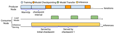Fig. 3. The High-level Architecture of Viper

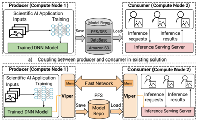Fig. 4. Lists of Viper's APIs

Viper's high-level architecture is illustrated in Figure 3. It serves as an I/O library and provides a set of APIs (e.g., save_weights() and load_weights() in Figure 4) for producers and consumers to interact with it. Viper includes four major components: a Checkpoint Callback, an Inference Performance Predictor, a Model Weights Handler, and a Notification Module. The Checkpoint Callback is a custom callback used to monitor the training quality of each iteration during training. It is responsible for tracking the DNN model's training metrics (e.g., training loss/accuracy of each iteration), capturing the DNN model's current state, and triggering model updates at specified checkpoints. Before starting training in the producer, a Checkpoint Callback object is created and added to the callback list of model.fit(). The Inference Performance Predictor is responsible for finding a near-optimal checkpoint schedule to balance the trade-off between training slowdown and inference quality improvement. It can estimate the cumulative inference quality over a set of inferences using the predicted training quality and generate a near-optimal checkpoint schedule using the specified algorithm. The predicted training quality is obtained through a learning curve function fitted using the training quality observed during the warm-up stage. Model Weights Handler is a memory-first engine to accelerate the delivery of checkpoints between producer and consumer. It is responsible for processing the save/load requests from Checkpoint Callback and the consumer respectively, and determining the most suitable data transfer strategy for delivering the model. The Notification Module is responsible for actively notifying consumers about DNN model updates, avoiding frequent polling of the model repository to detect changes and reducing the model update latency. Viper achieves objective 1 by the Inference Performance Predictor, and objective 2 by combining Model Weights Handler with Notification Module.

Figure 3 also depicts the flow of model updates between a producer and a consumer. As shown in the figure, the producer and the consumer operate concurrently. Before its execution, the producer creates a callback object by setting a configurable initial model update interval and then appends it to the callback list of model.fit(). When a model update is triggered by Checkpoint Callback, Model Weights Handler will select a suitable location for saving the model checkpoint and store the metadata (e.g., model name, version, location, and file path) to the Metadata DB (a shared in-memory database, e.g., Redis). The checkpoint is asynchronously saved to the chosen location (e.g., GPU memory, Host memory, or PFS). Following this, the Model Weights Handler puts a model update message to the Notification Module, allowing the producer to proceed to train the subsequent iterations. Upon receiving the update message, the Notification Module immediately notifies the consumer. The consumer, in response, sends a load request to retrieve the new checkpoint. To do this, Model Weights Handler fetches the model's location from the Metadata DB, reads the checkpoint from the corresponding location, and then returns the new model to the consumer. Once getting the new model, the consumer will seamlessly replace the previous model with this new one and serve incoming inference queries with the latest model.

On the consumer side, Viper overlaps the I/O involved in receiving an updated model and the inference serving using a double buffering technique: the updated model is written to an alternative copy, while the primary copy is used to serve inferences. When the I/O to the alternative copy is finished, then the primary copy and alternative copy are swapped atomically, which has a negligible overhead that causes imperceptible downtime, thus avoiding any negative impact on the inference serving rate.

4.3 Optimized Checkpointing Schedule

Viper builds an Inference Performance Predictor (IPP) to find a near-optimal checkpoint schedule to balance the trade-off between training slowdown and inference quality improvement. The IPP can estimate the cumulative inference quality over a specified period based on given input parameters (e.g., start iteration, stop iteration, number of inferences, training quality in the warm-up stage, and other constant parameters). The IPP depends on a Training Loss Predictor (TLP) and a Cumulative Inference Loss Predictor (CILP) to predict the cumulative inference quality. Without completing the entire training, IPP can identify and generate a checkpoint schedule that maximizes cumulative inference quality while not adding more overhead on training based on the specified algorithm. This schedule is the near-optimal checkpoint schedule.

The design of IPP relies on the following assumptions:

• (1) The training quality (e.g., loss/accuracy) of the DNN model can be predicted as a function of the number of training iterations.
• (2) The training quality (e.g., loss/accuracy) of a DNN model can be used as a proxy to estimate the inference quality.

The first one comes from the study of Domhan et al. [7], which indicates that the learning curve can describe the performance of an iterative machine learning algorithm as a function of the number of training iterations or its training time. A set of parametric fundamental functions used for modeling learning curves are offered in studies [26]. The second one is based on observations that the training quality curve and inference quality curve usually exhibit similar trends for traditional DNN models. Thus, it is justifiable to treat the training quality of a checkpoint as its inference quality for simplicity.

First, Viper introduces a TLP to estimate the training quality at a specific iteration 𝑥. Although several factors like model architecture, hyperparameters, and the choice of optimizer may influence the training quality (e.g., training loss/accuracy) of a DNN model, Viper assumes that the training application often uses DNN models that are already optimized in terms of architecture, hyperparameters, and optimizer. Moreover, the training loss curves observed in existing DNN models usually exhibit a stable and similar trend. As such, it is reasonable to model the training loss curve with a function and predict how the training converges.

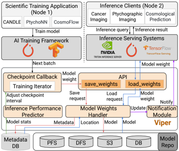Fig. 5. Fitting the learning curve for TC1 with the warmup training loss using four functions (the end of warm-up is marked with a vertical dotted line)

Fig. 6. TC1 training time and inference time per iter/req

Viper models the training loss learning curve using functions Exp2 (𝑎𝑒^-𝑏𝑥), Exp3 (𝑎𝑒^-𝑏𝑥 + 𝑐), Lin2 (𝑎𝑥 + 𝑏), and Expd3 (𝑐 - (𝑐 - 𝑎)𝑒^-𝑏𝑥), a subset of functions documented in the literature [26]. Viper chooses them as they show a decreasing trend, aligning with the performance trend observed in training loss. Viper utilizes the warm-up stage training loss to fit those learning curve functions and selects the most suitable one as its 'TLP' to predict future training loss. For instance, when modeling the training loss curve of the CANDLE-TC1, Exp3 is the best curve function since it has minimal Mean Squared Error (MSE). TLP is defined as: 𝑙𝑜𝑠𝑠_𝑝𝑟𝑒𝑑(𝑥) = 𝑎 ∗ 𝑒𝑥𝑝(-𝑏 ∗ 𝑥) + 𝑐, where 𝑥 represents the training iteration ID, while parameters 𝑎, 𝑏, and 𝑐 are used to control the learning curve shape. Certainly, users can define a custom predictor tailored to its specific training metric and replace the TLP with a different predictor.

There is a one-to-one mapping between the training iteration number and the training time, it is easy to map a given time 𝑡_𝑘 to a training iteration 𝑥′ if we know the training time of each iteration 𝑡_𝑡𝑟𝑎𝑖𝑛, the checkpoint interval 𝑐𝑘𝑝𝑡_𝑖, and the stall time 𝑡_𝑝 caused by checkpointing on the producer side. Obviously, 𝑡_𝑡𝑟𝑎𝑖𝑛 remains consistent throughout the training. This assertion is empirically validated by executing a training application for a single epoch and measuring 𝑡_𝑡𝑟𝑎𝑖𝑛 within that epoch (See Figure 6). The stall time 𝑡_𝑝 can be derived as 𝑡_𝑝 = 𝑠_𝑚𝑜𝑑𝑒𝑙 / 𝑏𝑤_𝑤𝑟𝑖𝑡𝑒, in which 𝑠_𝑚𝑜𝑑𝑒𝑙 refers to the DNN model size and 𝑏𝑤_𝑤𝑟𝑖𝑡𝑒 is the I/O bandwidth of writing a DNN model

checkpoint to the corresponding storage (e.g., GPU memory, Host memory, or PFS). For any given DNN model architecture, 𝑠_𝑚𝑜𝑑𝑒𝑙 remains consistent throughout the training process. It can be determined using two common methods: 1) serializing and saving the model as a file and getting the model size by checking the file size; 2) counting the number of parameters in the model and getting the model size by calculating the space needed for storing these parameters. In Viper, we already have the initial checkpoint file after the warmup stage, so we get the model size by checking the file size. Theoretically, the I/O bandwidth 𝑏𝑤_𝑤𝑟𝑖𝑡𝑒 remains constant, but in practice it tends to fluctuate. We obtain it by measuring the current I/O bandwidth of the corresponding storage in the system. Then we can convert the training time 𝑡_𝑘 into a training iteration ID 𝑥′ based on the input checkpoint interval 𝑐𝑘𝑝𝑡_𝑖 through formula:

where

Hence, the training quality observed at the time 𝑡_𝑘 is identical to that at training iteration 𝑥′, expressed as 𝑙𝑜𝑠𝑠_𝑝𝑟𝑒𝑑(𝑔𝑒𝑡_𝑖𝑡𝑒𝑟𝑠(𝑡_𝑘, 𝑐𝑘𝑝𝑡_𝑖)).

Next, we estimate the cumulative inference quality over a fixed duration 𝑡_𝑚𝑎𝑥. Here, the cumulative inference quality is determined by the sum of the inference losses for all requests executed within the interval [0, 𝑡_𝑚𝑎𝑥], which is called Cumulative Inference Loss (CIL). Viper introduces a CILP to estimate the CIL, where a lower value means a better prediction. The CILP uses the training loss of a checkpoint as the inference loss of that checkpoint based on Assumption 2. The consumer can handle inference requests while simultaneously loading the new model, since Viper segregates the inference serving thread from the model updating thread in its implementation. Assume that the timing of each inference request, denoted as 𝑡_𝑖𝑛𝑓𝑒𝑟, remains constant, which can be validated by performing a set of inferences in the consumer (Figure 6). The overhead for loading a new model on the consumer side, denoted as 𝑡_𝑐, is calculated through 𝑡_𝑐 = 𝑠_𝑚𝑜𝑑𝑒𝑙 / 𝑏𝑤_𝑟𝑒𝑎𝑑, where 𝑏𝑤_𝑟𝑒𝑎𝑑 represents the I/O bandwidth of reading a DNN model from the corresponding storage. It is measured using the same approach for getting 𝑏𝑤_𝑤𝑟𝑖𝑡𝑒. At this point, CILP calculates CIL over a fixed duration 𝑡_𝑚𝑎𝑥 using the following formula:

where

The goal of the IPP is to find a near-optimal checkpoint schedule to maximize the cumulative inference quality over a fixed duration while adding less overhead on training runtime. Here, maximizing the cumulative inference quality over a fixed duration means minimizing the CIL over a fixed duration. Therefore, the formula of CILP

1: function CIL ( 𝑖𝑛𝑡𝑒𝑟 , 𝑙𝑜𝑠𝑠 , 𝑐𝑘𝑝𝑡 _ 𝑣𝑒𝑟 , 𝑟𝑒𝑚 _ 𝑖𝑛𝑓 𝑒𝑟𝑠 ) 2: if 𝑐𝑘𝑝𝑡 _ 𝑣𝑒𝑟 == 1 then 3: 𝑖𝑛𝑓 𝑒𝑟𝑠 ←⌊ 𝑖𝑛𝑡𝑒𝑟 ∗ 𝑡 𝑡𝑟𝑎𝑖𝑛 + 𝑡 𝑝 + 𝑡 𝑐 𝑡 𝑖𝑛𝑓 𝑒𝑟 ⌋ ; 4: else 5: 𝑖𝑛𝑓 𝑒𝑟𝑠 ←⌊ 𝑖𝑛𝑡𝑒𝑟 ∗ 𝑡 𝑡𝑟𝑎𝑖𝑛 + 𝑡 𝑝 𝑡 𝑖𝑛𝑓 𝑒𝑟 ⌋ ; 6: end if 7: 𝑖𝑛𝑓 𝑒𝑟𝑠 ← 𝑚𝑖𝑛 ( 𝑖𝑛𝑓 𝑒𝑟𝑠,𝑟𝑒𝑚 _ 𝑖𝑛𝑓 𝑒𝑟𝑠 ) ; 8: 𝑒 _ 𝑖𝑡𝑒𝑟 -𝑠 _ 𝑖𝑡𝑒𝑟 ← 𝑙𝑜𝑠𝑠 ∗ 𝑖𝑛𝑓 𝑒𝑟𝑠 ; 9: return 𝑎𝑐𝑐 _ 𝑖𝑛𝑓 𝑒𝑟 _ 𝑙𝑜𝑠𝑠 , 𝑖𝑛𝑓 𝑒𝑟𝑠 ; 10: end function

Algorithm1 Calculate the Total Inference Losses within an Interval

used for determining a near-optimal checkpoint schedule is:

Based on the assumptions and the mathematical formulation of the IPP, we propose and implement two algorithms to determine the near-optimal checkpoint schedule: (1) a fixed-interval schedule, which assumes a regular checkpoint interval and whose goal is to find the near-optimal checkpoint frequency; (2) a greedy irregular-interval schedule, which assumes no constraint regarding when a checkpoint can be taken. The reason for proposing both algorithms are due to the following trade-off: a fixed-interval schedule makes it easier to optimize the asynchronous capture and transfer strategies for checkpoints, however at the expense of less flexibility in reducing the gap between the trained model on the producer and the model used for inferences on the consumer. Thanks to these two algorithms, the user has a choice of how to optimize this trade-off.

Optimal Schedule Algorithms: Algorithm 1 depicts the method used to calculate CIL within a given checkpoint interval, which is used by both fixed-interval and greedy algorithms. It utilizes two different equations (line 3 and line 5) for the first model updates and the remaining model updates since 𝑡_𝑐 overlaps with the next training iteration (see Figure 1). The aforementioned mathematical IPP describes how to predict a near-optimal regular interval checkpoint schedule to achieve objective 1. The fixed-interval algorithm is illustrated in Algorithm 2. It traverses all possible checkpoint intervals and chooses the one with the minimal CIL as the near-optimal checkpoint interval. However, the fixed-interval method overlooks the potential inference quality improvement between two consecutive checkpoints, possibly resulting in multiple updates with negligible improvement. To mitigate this problem, the greedy algorithm for predicting an irregular update interval checkpoint schedule is employed (see Algorithm 3). This algorithm performs a checkpoint exclusively when the improvement between the training loss of the current iteration and that of the preceding checkpoint surpasses a specified threshold (line 8). This threshold is determined during a warm-up phase by calculating the mean and standard deviation of the differences between consecutive training losses; the threshold is then set as the sum of this mean and standard deviation.

4.4 Accelerating Model Data Transfer

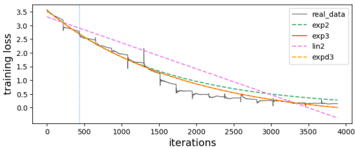Fig. 7. Viper's memory-first transfer engine

Viper creates an asynchronous memory-first model transfer engine, Model Weights Handler, to accelerate model movement between producer and consumer. During training, the producer can cache the DNN model in alternative locations, such as GPU memory, Host memory, local storage devices, or PFS, thanks to the multi-tiered storage architecture inherent in modern supercomputing compute

Algorithm 2 Fixed Interval Schedule Algorithm

Input: 𝑠 _ 𝑖𝑡𝑒𝑟 , 𝑒 _ 𝑖𝑡𝑒𝑟 , 𝑡𝑜𝑡𝑎𝑙 _ 𝑖𝑛𝑓 𝑒𝑟𝑠 Output: Anear-optimal checkpoint schedule 𝑏𝑒𝑠𝑡 _ 𝑖𝑛𝑡𝑒𝑟 1: 𝑚𝑖𝑛 _ 𝑙𝑜𝑠𝑠, 𝑏𝑒𝑠𝑡 _ 𝑖𝑛𝑡𝑒𝑟, 𝑚𝑎𝑥 _ 𝑖𝑛𝑡𝑒𝑟 ← 𝐼𝑛𝑓 𝑖𝑛𝑖𝑡𝑒, 𝑁𝑜𝑛𝑒,𝑒 _ 𝑖𝑡𝑒𝑟 -𝑠 _ 𝑖𝑡𝑒𝑟 2: for 𝑖 ← 1 ,𝑚𝑎𝑥 _ 𝑖𝑛𝑡𝑒𝑟 + 1 do 3: 𝑡 _ 𝑙, 𝑟𝑒𝑚 ← 0 , 𝑡𝑜𝑡𝑎𝑙 _ 𝑖𝑛𝑓 𝑒𝑟𝑠 ; 4: 𝑝 _ 𝑙 ← p_training_loss ( 𝑠 _ 𝑖𝑡𝑒𝑟 ) ; 5: 𝑐 _ 𝑖𝑡𝑒𝑟, 𝑐𝑘𝑝𝑡 _ 𝑣𝑒𝑟 ← 𝑠 _ 𝑖𝑡𝑒𝑟 + 𝑖, 1; 6: while 𝑐 _ 𝑖𝑡𝑒𝑟 < = 𝑒 _ 𝑖𝑡𝑒𝑟 do 7: 𝑖 _ 𝑙, 𝑖𝑛𝑓 𝑒𝑟𝑠 ← CIL ( 𝑖,𝑝 𝑙 ,𝑐𝑘𝑝𝑡 _ 𝑣𝑒𝑟,𝑟𝑒𝑚 ) ; 8: 𝑡 _ 𝑙, 𝑟𝑒𝑚 ← 𝑡 _ 𝑙 + 𝑖 _ 𝑙, 𝑟𝑒𝑚 -𝑖𝑛𝑓 𝑒𝑟𝑠 ; 9: 𝑝 _ 𝑙 ← p_training_loss ( 𝑐 _ 𝑖𝑡𝑒𝑟 ) ; 10: 𝑐 _ 𝑖𝑡𝑒𝑟, 𝑐𝑘𝑝𝑡 _ 𝑣𝑒𝑟 ← 𝑐 _ 𝑖𝑡𝑒𝑟 + 𝑖, 𝑐𝑘𝑝𝑡 _ 𝑣𝑒𝑟 + 1; 11: end while 12: 𝑡 _ 𝑙 ← 𝑡 _ 𝑙 + 𝑝 _ 𝑙 ∗ 𝑟𝑒𝑚 ; 13: if 𝑡 _ 𝑙 < 𝑚𝑖𝑛 _ 𝑙𝑜𝑠𝑠 then 14: 𝑚𝑖𝑛 _ 𝑙𝑜𝑠𝑠, 𝑏𝑒𝑠𝑡 _ 𝑖𝑛𝑡𝑒𝑟 ← 𝑡 _ 𝑙, 𝑖 ; 15: end if 16: end for 17: return 𝑏𝑒𝑠𝑡 _ 𝑖𝑛𝑡𝑒𝑟

Algorithm 3 Irregular Interval Schedule Algorithm: Greedy

Input: 𝑠 _ 𝑖𝑡𝑒𝑟 , 𝑒 _ 𝑖𝑡𝑒𝑟 , 𝑡𝑜𝑡𝑎𝑙 _ 𝑖𝑛𝑓 𝑒𝑟𝑠 , 𝑡ℎ𝑟𝑒𝑠ℎ Output: Anear-optimal checkpoint schedule 𝑏𝑒𝑠𝑡 _ 𝑠𝑐ℎ𝑒𝑑 1: 𝑏𝑒𝑠𝑡 _ 𝑠𝑐ℎ𝑒𝑑, 𝑝 _ 𝑖𝑡𝑒𝑟 ←[] , 𝑠 _ 𝑖𝑡𝑒𝑟 2: 𝑝 _ 𝑙 ← p_train_loss ( 𝑠 _ 𝑖𝑡𝑒𝑟 ) ; 3: 𝑖, 𝑐𝑘𝑝𝑡 _ 𝑣, 𝑟𝑒𝑚 ← 𝑠 _ 𝑖𝑡𝑒𝑟 + 1 , 1 , 𝑡𝑜𝑡𝑎𝑙 _ 𝑖𝑛𝑓 𝑒𝑟𝑠 ; 4: while 𝑖 < = 𝑒 _ 𝑖𝑡𝑒𝑟 do 5: 𝑐 _ 𝑙 ← p_train_loss ( 𝑖 ) 6: if ( 𝑐 _ 𝑙 < 𝑝 _ 𝑙 ) ∧ ( 𝑎𝑏𝑠 ( 𝑐 _ 𝑙 -𝑝 _ 𝑙 ) > 𝑡ℎ𝑟𝑒𝑠ℎ ) then 7: 𝑖 _ 𝑙, 𝑖𝑛𝑓 𝑒𝑟𝑠 ← CIL ( 𝑖 -𝑝 _ 𝑖𝑡𝑒𝑟,𝑝 _ 𝑙,𝑐𝑘𝑝𝑡 _ 𝑣,𝑟𝑒𝑚 ) ; 8: 𝑝 _ 𝑙, 𝑝 _ 𝑖𝑡𝑒𝑟, ← 𝑐 _ 𝑙, 𝑖 ; 9: 𝑏𝑒𝑠𝑡 _ 𝑠𝑐ℎ𝑒𝑑.𝑎𝑝𝑝𝑒𝑛𝑑 ( 𝑖 ) ; 10: 𝑖, 𝑐𝑘𝑝𝑡 _ 𝑣, 𝑟𝑒𝑚 ← 𝑖 + 1 , 𝑐𝑘𝑝𝑡 _ 𝑣 + 1 , 𝑟𝑒𝑚 -𝑖𝑛𝑓 𝑒𝑟𝑠 11: end if 12: end while 13: return 𝑏𝑒𝑠𝑡 _ 𝑠𝑐ℎ𝑒𝑑

;

nodes. Model Weights Handler utilizes the cached DNN models on the producer's end and creates a direct communication channel to deliver the model data between producer and consumer.

There are two direct communication channels: direct GPU-to-GPU memory and direct Host-to-Host memory. Viper is designed to be generic, ensuring compatibility across various GPU vendors. It prefers GPU-to-GPU communication when it is available (e.g., NVIDIA's GPUDirect Remote Direct Memory Access (RDMA) and GPUDirect Peer-to-Peer, along with AMD's ROCm RDMA) due to the high I/O bandwidth. To this end, it relies on the Message Passing Interface (MPI) library by taking advantage of standardized high-level vendor-optimized communication primitives (MPI_Send and MPI_Recv), which are supported by popular implementations: OpenMPI, MVAPICH2, and Cray MPICH. When direct GPU-to-GPU communication is not available, Viper falls back to host-to-host RDMA transfer. In this case, a DNN model snapshot is first transferred from the GPU memory to the Host memory (which blocks the training until completion). Then, the snapshot residing in the producer's Host memory is sent to the consumer's Host memory through the InfiniBand (IB) network. Once received, the consumer will update its loaded model's tensors by copying the data from the Host memory to the responding GPU memory (e.g., using the CUDA's cudaMemcpyAsync API). Although this method involves extra overheads of using the host memory as a staging area (on both the producer and the consumer), it is still significantly faster than writing to and reading from a repository such as a PFS.

Figure 7 showcases how Model Weights Handler handles the save/load requests and routes the model using distinct transfer strategies. When processing the save request from the producer, Model Weights Handler first utilizes the Transfer Selector to select a proper transfer strategy based on the existing workload on the storage and then delivers the model data using the selected transfer strategy. In Viper, GPU-to-GPU memory and Host-to-Host memory communications only buffer and transfer the latest DNN model due to the limited size of GPU memory and Host memory. For fault tolerance, all historical DNN models are flushed to the PFS through a background thread to minimize the impact on training. Flushing the models to PFS may increase memory utilization. However, the DNN models targeted by this work are small and can fit in the GPU memory. Therefore, an extra copy in the Host memory for flushing is not a problem.

Viper utilizes a lightweight publish-subscribe notification module (based on Redis) to reduce model discovery latency by proactively informing consumers of model updates. Unlike state-of-the-art approaches (e.g., NVIDIA's Triton [19]), which periodically poll the model repository to check for updates (the minimal latency is 1ms), our approach achieves less than 1ms notification latency. Thus, when an updated model is available, it can be immediately transferred to the consumer without any delay caused by polling. This reduces the transfer time, allowing inferences to utilize the updated model more quickly, thereby enhancing the overall quality of the inferences.

5 EVALUATIONS

5.1 Experimental Setup

Testbed. Our experiments were conducted on ALCF's Polaris system, consisting of 560 compute nodes. Each node has an AMD Zen 3 (Milan) CPU (64 threads), 4 × A100 40GB GPUs interconnected via NVLink, and 512 GB DDR4 RAM. The nodes are interconnected using the Slingshot 10 network. Additionally, Lustre is used as the external storage, with a aggregated I/O bandwidth of 650 GB/s.

Software. Viper is implemented using Python and C++. The memory-first engine is implemented through C++ because Python's efficiency in multithreading is limited by Global Interpreter Lock (GIL). The IPP is implemented using Python. It is integrated as a plugin within Viper, allowing users to create alternative optimization algorithms to find the near-optimal checkpoint schedule. Viper exposes a set of Python APIs through nanobind-1.5.2 so that the producer and consumer can interact with it. We utilize MPICH and CUDA to build memory-to-memory communication channels, Tensorflow-2.9 for performing training and inferences, and Redis-7.4 as a database to store the DNN model metadata.

5.2 Applications and Metrics

Applications: CANDLE-NT3: Pilot1 benchmarks from the CANDLE [29] project aim to predict drug response based on molecular features of tumor cells and drug descriptors. NT3 within Pilot1 is a 1D convolutional network for classifying RNA-seq gene expression profiles into normal or tumor tissue. It follows a traditional convolutional model structure with multiple 1D convolutional layers interleaved with pooling layers followed by final dense layers. It uses SGD (stochastic gradient descent) optimizer. Its training dataset contains 1120 samples, with an additional 280 samples for test.

CANDLE-TC1: TC1, another Pilot1 benchmark, is also a 1D convolutional network but classifies RNA-seq gene expression profiles into 18 balanced tumor types. It adopts an architecture akin to NT3 and utilizes the same optimizer. Its training dataset includes 4320 samples, while the test dataset has 1080 samples.

PtychoNN: PtychoNN [1] is a neural network that simultaneously predicts real-space amplitude and phase from input diffraction data alone. Its architecture includes three parts: an encoder that learns a representation (encoding) in the feature space of the x-ray diffraction data, and two decoders that learn to map from the encoding to real-space amplitude and phase respectively. It selects Adam as the optimizer. Its training dataset contains 16100 samples, while the test dataset has 3600 samples.

Metrics: We measured the end-to-end model update latency by summing the checkpointing time (producer side) and the delivery/loading time (consumer side). To assess IPP, we use CIL as the metric, since a single scalar metric makes it easy to compare different approaches. CIL is the total inference loss accumulated across a set number of inferences. A lower CIL indicates a better result. For NT3 and TC1, the inference loss is measured through Cross-Entropy loss, the difference between the ground truth and the prediction. PtychoNN uses the MeanAbsoluteError loss to measure its inference loss. We executed all tests three times and reported the average value.

5.3 Results: Model Update Latency

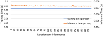Fig. 8. The end-to-end model update latency across different data transfer strategies: (a) CANDLE-NT3.A Model (Size: 600MB), (b) CANDLE-TC1 Model (Size: 4.7GB), (c) PtychoNN Model (Size: 4.5GB)

We conducted two tests to assess our model transfer method: (1) evaluating the end-to-end model update latency across different strategies; and (2) evaluating the benefits of using a low-latency model update method. In these tests, we deploy a producer (training application) and a consumer (synthetic inference system) on separate nodes to avoid node-local caching. They are running in parallel after the warm-up period.

End-to-End Model Update Latency: We first study the end-to-end model update latency using three transfer strategies: PFS, Host-to-Host memory, and GPU-to-GPU memory. To do this, we compared six different approaches for data sharing between a producer and a consumer: h5py(baseline), Viper-PFS, Viper-Sync(Host Memory), Viper-ASync(Host Memory), Viper-Sync(GPU Memory), and Viper-ASync(GPU Memory). Here h5py means using h5py API to transfer the checkpoint through PFS while Viper-PFS refers to using Viper's API; Viper-Sync and Viper-Async indicate synchronous and asynchronous model transfers, respectively, through either GPU or Host memory. The goal is to show that Viper can significantly reduce the model update latency compared with the baseline. We analyzed the model update latency of three DNN models: NT3.A (600 MB), TC1 (4.7 GB), and PtychoNN (4.5 GB).

Figure 8a depicts the results of NT3.A, in which the baseline latency is 1.5 seconds. The results reveal that both GPU-to-GPU memory and Host-to-Host memory methods can achieve better performance. Specifically, GPU-to-GPU memory outperforms the baseline by 12x (using Viper-Async), saving 1.4 seconds of latency. Host-to-Host memory outperforms the baseline by 4x (using ViperAsync), saving 1.1 seconds of latency. The improvement is attributed to the high I/O bandwidth of the fast memory tiers and the highspeed network. We also noticed that Viper-PFS saves 0.4 seconds of latency, making it about 1.3x faster than the baseline. That is because Viper only writes the model weights and closely related metadata into the file, avoiding some unnecessary metadata added by h5py. Moreover, we also observed that Viper-Async is a bit slower than Viper-sync. It is because Viper-Async handles data transfer with a separate thread to reduce the interruption time on training, which requires an extra copy and increases latency compared with ViperSync. Although Viper-Sync can get lower latency, it increases the training duration due to the blocking of data delivery.

Figure 8b shows the result of TC1, a large-size model. The baseline latency is 8.0 seconds, greater than the baseline for the smaller model. The findings once more highlight that GPU-to-GPU memory communication offers 9x improvement over the baseline, but this time it saves 7.1 seconds. Host-to-Host memory communication achieves 3x improvement compared to the baseline, saving 5.6 seconds of latency. Note that the greater model size makes the observed latency reduction greater. Larger models see more benefit from the GPU-to-GPU or Host-to-Host memory transfer methods.

Figure 8c describes the result of PtychoNN. Its baseline latency is 8.3 seconds, which is a bit slower than the baseline for TC1. That is because PtychoNN's model architecture is different from TC1, which takes more time to load the model. Once more, we observed that Viper significantly reduces the end-to-end model update latency compared with the baseline. Specifically, GPU-to-GPU memory reduces the latency by a factor of 15x compared to the baseline, and Host-to-Host memory is at least 4x less than the baseline. Viper-PFS also reduces the latency by a factor of 1.2x.

All findings suggest that Viper enhances model data transfer, particularly with direct communication methods. While our results are based on the average latency between one producer and one consumer, these insights are likely applicable on a larger scale. This will be a focus of our future work when exploring data transfer between multi-producers and multi-consumers for large models.

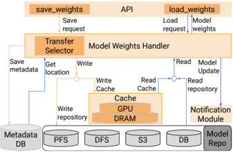Fig. 9. Impact of a low-latency model update on inference and training performance (update interval: epoch boundary)

Benefits of Low-latency Model Update. This test illustrates the cumulative inference quality improvement achieved using a low-latency transfer strategy and quantifies the overhead added to training using different strategies. We test with TC1 model and set its update interval at the epoch boundary (216 iterations). We measure the Cumulative Inference Loss (CIL) over 50,000 inferences and the training overhead caused by model updates across three strategies.

In Figure 9, the blue bar demonstrates the CIL across various strategies, and the orange line represents the training overhead incurred by checkpointing under different transfer strategies. We can see a notable trend: for the same number of model updates (16 checkpoints), both GPU-to-GPU memory and Host-to-Host memory exhibit lower CIL and less training overhead than PFS. A lower value means better performance. For instance, the overhead of GPU-to-GPU memory is 1s, which is negligible compared to PFS (60s). Although Host-to-Host memory introduces more overhead (22s) compared to GPU-to-GPU memory, it is still much better than PFS. This is because the I/O access to GPU memory and Host memory is much faster than PFS. While 16 checkpoints provide 60 seconds of overhead reduction between PFS and GPU, more checkpoints will compound this so that an application performing 2000 checkpoints should see about two hours of training overhead reduction. This could be invaluable time in a time-constrained scenario. In addition, the consumer handles inferences at a consistent rate, as evidenced by the uniform inference request time shown in Figure 6 (§ 4.3). In this context, utilizing a low-latency method to transmit the model can obtain minimal CIL because it enables the consumer side to process more inferences using the most recent models. Conversely, if there is insufficient GPU or Host memory and the model is transferred through PFS, there is a marked increase in CIL. This rise is attributed to more inferences being served by older models compared with direct communication channels. Thus, delivering a model with low latency is required and useful as it improves the cumulative inference quality and minimizes the overhead on training time.

5.4 Results: Inference Performance Predictor

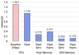Fig. 10. Cumulative inference loss over a fixed number of inferences using different checkpoint schedule methods: (a) NT3.B over 25,000 inferences, (b) TC1 over 50,000 inferences, (c) PtychoNN over 40,000 inferences

Table 1: Checkpoints and training overhead

	Num of Checkpoints	Num of Checkpoints	Num of Checkpoints	Training Overhead (s)	Training Overhead (s)	Training Overhead (s)
	Baseline	Fixed-inter	Adapt-inter	Baseline	Fixed-inter	Adapt-inter
NT3.B	7	49	40	0.107	0.372	0.353
TC1	16	128	63	1.29	3.437	2.579
PtychoNN	13	16	6	0.39	0.48	0.18

This experiment evaluates the Cumulative Inference Loss (CIL) over a fixed number of inferences using the GPU-to-GPU memory transfer strategy based on three checkpoint schedules: epoch-boundary (Baseline), fixed-interval, and adaptive-interval. We aim to show that the checkpoint schedule identified by IPP can achieve lower CIL compared to the baseline. The fixed and adaptive checkpoint schedules represent the ones found using the fixed-interval and the greedy algorithm respectively (§ 4.3). The fixed-interval algorithm describes a naive method of finding the near-optimal schedule. We run with three applications: NT3.B, TC1, and PtychoNN (real-life application).

Figure 10a displays the results of NT3.B (1.7GB) across 25,000 inferences across different checkpoint schedules. Compared with the baseline, the adaptive-interval schedule reduces the CIL from 3.8k to 3.0k, while the fixed-interval schedule reduces it from 3.8k to 3.6k. This aligns with our expectations. As indicated in Table 1, although our predicted schedules yield more model updates than the baseline, they achieve lower CIL without adding too much training overhead, about 0.25s when using the adaptive method in contrast to the baseline. The adaptive method's efficacy stems from its capability to adjust the update interval according to the training converging rate. This can produce more frequent updates initially because of the rapid decline in training loss, and less frequent updates as it approaches the convergence point due to the gradual stabilization of training loss.

Figure 10b shows the outcomes for TC1 (4.7GB) over 50,000 requests. With a fixed number of inference requests, both the fixed-interval and the adaptive-interval schedules lower the CIL to 30.6k and 30.4k, respectively, from the 32.8k (baseline). Although the disparity in CIL between the fixed-interval and the adaptive-interval schedule is small (0.2k), the number of checkpoints using the adaptive method is roughly half compared to those produced using the fixed-interval approach (Table 1). This reconfirms that utilizing an adaptive interval schedule can help us get lower CIL.

Similarly, Figure 10c depicts the results of PtychoNN (4.5GB) over 40,000 inference requests with the same checkpoint schedules. We observed that the fixed-interval and the adaptive-interval schedules reduce the CIL from the baseline of 66.2k to 52.9k and 45.1k respectively. Once more, the adaptive-interval schedule allows us to get better CIL with fewer checkpoints compared to the fixed-interval approach (as shown in Table 1). This indicates Viper's capability to identify the near-optimal checkpoint schedule for actual applications.

6 CONCLUSION AND FUTURE WORK

This work proposes Viper, an I/O framework that determines a viable checkpoint schedule and accelerates the scheduled DNN model checkpoints delivery from producer to consumer. To identify the near-optimal schedule, Viper designs two algorithms based on an intelligent inference performance predictor that predicts the CIL based on the predicted training loss and checkpoint delivery overhead. Viper creates an asynchronous memory-first model transfer engine alongside a push-based notification module to accelerate checkpoint delivery. Experimental results show that Viper can reduce the model update latency by ≈ 9x with GPU-to-GPU strategy and ≈ 3x with Host-to-Host strategy. Furthermore, our predictor-driven schedule also contributes to improved cumulative inference quality.

Currently, Viper primarily targets DNN models that can fit in the memory of a single GPU. Given the increasing popularity of model parallelism, especially in the context of LLMs and transformers, we will extend our work with support for a multi-producer, multi-consumer pattern in which we allow the DNN model to be sharded in different ways during the training and inferences (e.g. by mixing tensor, pipeline, and data parallelism).

ACKNOWLEDGMENTS

This material is based upon work supported by the U.S. Department of Energy (DOE), Office of Science, Office of Advanced Scientific Computing Research, under Contracts DE-AC02-06CH11357 and DE-AC02-05CH11231. Additionally, this work is partially supported by the National Science Foundation (NSF), Office of Advanced Cyberinfrastructure, under Grants CSSI-2104013 and Core-2313154.

REFERENCES

[1] Anakha V Babu, Tekin Bicer, Saugat Kandel, Tao Zhou, Daniel J Ching, Steven Henke,Siniša Veseli, Ryan Chard, Antonino Miceli, and Mathew Joseph Cherukara. 2023. AI-assisted automated workflow for real-time x-ray ptychography data analysis via federated resources. arXiv preprint arXiv:2304.04297 (2023).

[2] Nathan Baker, Frank Alexander, Timo Bremer, Aric Hagberg, Yannis Kevrekidis, Habib Najm, Manish Parashar, Abani Patra, James Sethian, Stefan Wild, et al. 2019. Workshop report on basic research needs for scientific machine learning: Core technologies for artificial intelligence . Technical Report. USDOE Office of Science (SC), Washington, DC (United States).

[3] Dimitri Bourilkov. 2019. Machine and deep learning applications in particle physics. International Journal of Modern Physics A 34, 35 (2019), 1930019.

[4] Fahim Chowdhury, Yue Zhu, Todd Heer, Saul Paredes, Adam Moody, Robin Goldstone, Kathryn Mohror, and Weikuan Yu. 2019. I/o characterization and performance evaluation of beegfs for deep learning. In Proceedings of the 48th International Conference on Parallel Processing . 1-10.

[5] Daniel Crankshaw, Xin Wang, Giulio Zhou, Michael J Franklin, Joseph E Gonzalez, and Ion Stoica. 2017. Clipper: A Low-Latency Online Prediction Serving System.. In NSDI , Vol. 17. 613-627.

[6] Hariharan Devarajan, Anthony Kougkas, Huihuo Zheng, Venkatram Vishwanath, and Xian-He Sun. 2022. Stimulus: Accelerate Data Management for Scientific AI applications in HPC. In 2022 22nd IEEE International Symposium on Cluster, Cloud and Internet Computing (CCGrid) . IEEE, 109-118.

[7] Tobias Domhan, Jost Tobias Springenberg, and Frank Hutter. 2015. Speeding up automatic hyperparameter optimization of deep neural networks by extrapolation of learning curves. In Twenty-fourth international joint conference on artificial intelligence .

[8] Assaf Eisenman, Kiran Kumar Matam, Steven Ingram, Dheevatsa Mudigere, Raghuraman Krishnamoorthi, Krishnakumar Nair, Misha Smelyanskiy, and Murali Annavaram. 2022. Check-N-Run: a checkpointing system for training deep learning recommendation models. In 19th USENIX Symposium on Networked Systems Design and Implementation (NSDI 22) . 929-943.

[9] Raia Hadsell, Dushyant Rao, Andrei A Rusu, and Razvan Pascanu. 2020. Embracing change: Continual learning in deep neural networks. Trends in Cognitive Sciences 24, 12 (2020), 1028-1040.

[10] Junchen Jiang, Ganesh Ananthanarayanan, Peter Bodik, Siddhartha Sen, and Ion Stoica.2018. Chameleon:scalableadaptationofvideoanalytics.In Proceedingsofthe 2018 conference of the ACM special interest group on data communication . 253-266.

[11] Zhengchun Liu, Hemant Sharma, J-S Park, Peter Kenesei, Antonino Miceli, Jonathan Almer, Rajkumar Kettimuthu, and Ian Foster. 2022. BraggNN: fast X-ray Bragg peak analysis using deep learning. IUCrJ 9, 1 (2022), 104-113.

[12] Meghana Madhyastha, Robert Underwood, Randal Burns, and Bogdan Nicolae. 2023. DStore: A Lightweight Scalable Learning Model Repository with Fine-Grain Tensor-Level Access. In Proceedings of the 37th International Conference on Supercomputing . 133-143.

[13] Avinash Maurya, Robert Underwood, Mustafa Rafique, Franck Cappello, and Bogdan Nicolae. 2024. DataStates-LLM: Lazy Asynchronous Checkpointing for Large Language Models. In HPDC'24: The 33nd International Symposium on High-Performance Parallel and Distributed Computing . Pisa, Italy.

[14] Martial Mermillod, Aurélia Bugaiska, and Patrick Bonin. 2013. The stabilityplasticity dilemma: Investigating the continuum from catastrophic forgetting to age-limited learning effects. Frontiers in Psychology 4 (2013), 504.

[15] microsoft. 2023. ONNX Runtime: A cross-platform inference and training machine-learning accelerator . https://github.com/microsoft/onnxruntime

[16] Jayashree Mohan, Amar Phanishayee, and Vijay Chidambaram. 2021. CheckFreq: Frequent, Fine-Grained DNN Checkpointing.. In FAST , Vol. 21. 203-216.

[17] Bogdan Nicolae, Jiali Li, Justin M Wozniak, George Bosilca, Matthieu Dorier, and Franck Cappello. 2020. Deepfreeze: Towards scalable asynchronous checkpointing of deep learning models. In 2020 20th IEEE/ACM International Symposium on Cluster, Cloud and Internet Computing (CCGRID) . IEEE, 172-181.

[18] Bogdan Nicolae, Justin M Wozniak, Matthieu Dorier, and Franck Cappello. 2020. DeepClone: Lightweight State Replication of Deep Learning Models for Data Parallel Training. In CLUSTER'20: The 2020 IEEE International Conference on Cluster Computing . Kobe, Japan.

[19] NVIDIA. 2023. NVIDIA Triton Inference Server . https://docs.nvidia.com/ deeplearning/triton-inference-server/user-guide/docs/user_guide/architecture. html

[20] Christopher Olston, Noah Fiedel, Kiril Gorovoy, Jeremiah Harmsen, Li Lao, Fangwei Li, Vinu Rajashekhar, Sukriti Ramesh, and Jordan Soyke. 2017. Tensorflow-serving: Flexible, high-performance ml serving. arXiv preprint arXiv:1712.06139 (2017).

[21] pytorch. 2023. TorchServe: a flexible and easy to use tool for serving and scaling PyTorch models in production . https://github.com/pytorch/serve

[22] Stephan Rasp, Peter D Dueben, Sebastian Scher, Jonathan A Weyn, Soukayna Mouatadid, and Nils Thuerey. 2020. WeatherBench: a benchmark data set for data-driven weather forecasting. Journal of Advances in Modeling Earth Systems 12, 11 (2020), e2020MS002203.

[23] DongInShin, Young Jin Yu, Hyeong S Kim, Jae Woo Choi, Heon Y Yeom, et al. 2013. DynamicInterval Polling and Pipelined Post { I/O } Processing for { Low-Latency } Storage Class Memory. In 5th USENIX Workshop on Hot Topics in Storage and File Systems (HotStorage 13) .

[24] Chijun Sima, Yao Fu, Man-Kit Sit, Liyi Guo, Xuri Gong, Feng Lin, Junyu Wu, Yongsheng Li, Haidong Rong, Pierre-Louis Aublin, et al. 2022. Ekko: A { Large-Scale } Deep Learning Recommender System with { Low-Latency } Model Update. In 16th USENIX Symposium on Operating Systems Design and Implementation (OSDI 22) . 821-839.

[25] Robert Underwood, Meghana Madhyastha, Randal Burns, and Bogdan Nicolae. 2024. EvoStore: Towards Scalable Storage of Evolving Learning Models. In HPDC'24: The 33nd International Symposium on High-Performance Parallel and Distributed Computing . Pisa, Italy.

[26] Tom Viering and Marco Loog. 2022. The shape of learning curves: a review. IEEE Transactions on Pattern Analysis and Machine Intelligence (2022).

[27] Ricardo Vinuesa and Steven L Brunton. 2022. Enhancing computational fluid dynamics with machine learning. Nature Computational Science 2, 6 (2022), 358-366.

[28] Yingcan Wei, Matthias Langer, Fan Yu, Minseok Lee, Jie Liu, Ji Shi, and Zehuan Wang. 2022. A GPU-specialized Inference Parameter Server for Large-Scale Deep Recommendation Models. In Proceedings of the 16th ACM Conference on Recommender Systems . 408-419.

[29] Justin M Wozniak, Rajeev Jain, Prasanna Balaprakash, Jonathan Ozik, Nicholson T Collier, John Bauer, Fangfang Xia, Thomas Brettin, Rick Stevens, Jamaludin Mohd-Yusof,etal.2018. CANDLE/Supervisor:Aworkflowframeworkformachine learning applied to cancer research. BMCbioinformatics 19, 18 (2018), 59-69.

Cumulative Inference Loss

35.0k

30.0k

25.0k

20.0k

15.0k

10.0k

5.0k

0.0k

Cumulative Inference Loss

70.0k

60.0k

50.0k

40.0k

30.0k

20.0k

10.0k

0.0k

66.2k

52.9k